Effects of dataset height and width on DP sums

Differential privacy will work best on datasets that are “tall and skinny”: They have a lot of rows, but only a small number of columns under analysis. Having more rows means that the contribution of any particular row is smaller, and having fewer columns reveals less information for every row.

But how tall is tall enough? And how many columns is too many columns? In this notebook we’ll demonstrate the effects of DP on different kinds of datasets, so you you can make an informed decision about whether DP is an appropriate technology.

import matplotlib.pyplot as plt
import opendp.prelude as dp
import polars as pl

# The OpenDP team is working to vet the core algorithms.
# Until that is complete we need to opt-in to use these features.
dp.enable_features("contrib")

For this example, we’ll just use constant data, so the only variation in the results comes from the noise added by DP. We’ll make every value 5, perhaps in a range between 0 and 10. (But we’ll look at the effects of this range assumption later.)

def make_fives_lf(rows, cols):
    """
    Makes a lazyframe with the specified rows and column, filled with fives.
    """
    return pl.LazyFrame({f"col_{i + 1}": (5 for _ in range(rows)) for i in range(cols)})

These values will be constant in every example:

MAX_ROWS_LOG_10 = 5
MAX_COLS_LOG_2 = 5

Let’s see how well DP sums work on datasets of different dimensions:

def key(rows, cols):
    return f"{rows=} {cols=}"

def get_results_accuracies(plus_minus=5, epsilon=1.0):
    results = {}
    accuracies = {}

    for rows_log_10 in range(1, MAX_ROWS_LOG_10):
        rows = 10**rows_log_10
        for cols_log_2 in range(MAX_COLS_LOG_2):
            cols = 2**cols_log_2
            context = dp.Context.compositor(
                data=make_fives_lf(rows=rows, cols=cols),
                privacy_unit=dp.unit_of(contributions=1),
                privacy_loss=dp.loss_of(epsilon=epsilon, delta=0),
                split_by_weights=[1],
                margins=[
                    # We'll assume that we know the size of the dataset.
                    dp.polars.Margin(max_length=rows),
                ],
            )

            col_queries = [
                # Values are clipped by plus_minus.
                pl.col(f"col_{i + 1}").dp.sum((5 - plus_minus, 5 + plus_minus))
                for i in range(cols)
            ]
            query = context.query().select(*col_queries)
            accuracy = query.summarize(alpha=0.05)["accuracy"][0]

            k = key(rows, cols)
            accuracies[k] = accuracy
            print(key(rows, cols), accuracy)
            results[k] = query.release().collect()

    return results, accuracies

results, accuracies = get_results_accuracies()

rows=10 cols=1 30.444827940403663
rows=10 cols=2 60.408396122013016
rows=10 cols=4 120.32616602353652
rows=10 cols=8 240.15701939449175
rows=10 cols=16 479.8163825199104
rows=100 cols=1 30.444827940403663
rows=100 cols=2 60.408396122013016
rows=100 cols=4 120.32616602353652
rows=100 cols=8 240.15701939449175
rows=100 cols=16 479.8163825199104
rows=1000 cols=1 30.444827940403663
rows=1000 cols=2 60.408396122013016
rows=1000 cols=4 120.32616602353652
rows=1000 cols=8 240.15701939449175
rows=1000 cols=16 479.8163825199104
rows=10000 cols=1 30.444827940403663
rows=10000 cols=2 60.408396122013016
rows=10000 cols=4 120.32616602353652
rows=10000 cols=8 240.15701939449175
rows=10000 cols=16 479.8163825199104

def plot(results, accuracies):
    _fig, axs = plt.subplots(MAX_ROWS_LOG_10 - 1, MAX_COLS_LOG_2)

    for rows_log_10 in range(1, MAX_ROWS_LOG_10):
        rows = 10**rows_log_10
        for cols_log_2 in range(MAX_COLS_LOG_2):
            cols = 2**cols_log_2
            values = results[key(rows, cols)].to_dicts()[0].values()
            ax = axs[rows_log_10 - 1, cols_log_2]
            ax.bar(range(cols), values, yerr=accuracies[key(rows, cols)])
            ax.set_xticks([])
            ax.set_yticks(
                [0, rows * 5], labels=[0, rows * 5] if cols == 1 else ["", ""]
            )

    plt.show()

plot(results, accuracies)

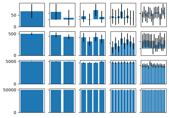
As you can see, with smaller numbers of rows, and larger numbers of columns, the accuracy of the sum declines: with each row making a larger contribution to the final statistic, more noise is necessary to hide individual contributions.

Are there strategies we can use to improve our results? Yes! Most obviously, make fewer queries. This about the questions that are really immportant to you, and your privacy budget can go farther.

Another option when working with sums or means is to adjust the clipping bounds. In this example we assumed the values could range between 0 and 10. What if we narrow the range? If there were outliers, the results would be biases, but if we are confident that values lie in a smaller range, we can get more accurate results.

results, accuracies = get_results_accuracies(
    plus_minus=1
)  # 4 to 6, instead of 0 to 10.

rows=10 cols=1 18.4535843760858
rows=10 cols=2 36.43837362866836
rows=10 cols=4 72.3923666086791
rows=10 cols=8 144.29254501101863
rows=10 cols=16 288.0889961837368
rows=100 cols=1 18.4535843760858
rows=100 cols=2 36.43837362866836
rows=100 cols=4 72.3923666086791
rows=100 cols=8 144.29254501101863
rows=100 cols=16 288.0889961837368
rows=1000 cols=1 18.4535843760858
rows=1000 cols=2 36.43837362866836
rows=1000 cols=4 72.3923666086791
rows=1000 cols=8 144.29254501101863
rows=1000 cols=16 288.0889961837368
rows=10000 cols=1 18.4535843760858
rows=10000 cols=2 36.43837362866836
rows=10000 cols=4 72.3923666086791
rows=10000 cols=8 144.29254501101863
rows=10000 cols=16 288.0889961837368

plot(results, accuracies)

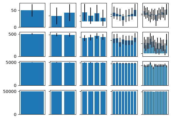
Another option is to use a larger or smaller privacy budget. If you have a large number of contributors, or a small number of queries, you might use an epsilon much less than 1 and still have sufficiently accurate results.

results, accuracies = get_results_accuracies(
    epsilon=0.05
)  # 1/20th of the original budget.

rows=10 cols=1 599.6458297114494
rows=10 cols=2 1198.792596921678
rows=10 cols=4 2397.0856625932033
rows=10 cols=8 4793.671559561389
rows=10 cols=16 9586.84323631028
rows=100 cols=1 599.6458297114494
rows=100 cols=2 1198.792596921678
rows=100 cols=4 2397.0856625932033
rows=100 cols=8 4793.671559561389
rows=100 cols=16 9586.84323631028
rows=1000 cols=1 599.6458297114494
rows=1000 cols=2 1198.792596921678
rows=1000 cols=4 2397.0856625932033
rows=1000 cols=8 4793.671559561389
rows=1000 cols=16 9586.84323631028
rows=10000 cols=1 599.6458297114494
rows=10000 cols=2 1198.792596921678
rows=10000 cols=4 2397.0856625932033
rows=10000 cols=8 4793.671559561389
rows=10000 cols=16 9586.84323631028

plot(results, accuracies)

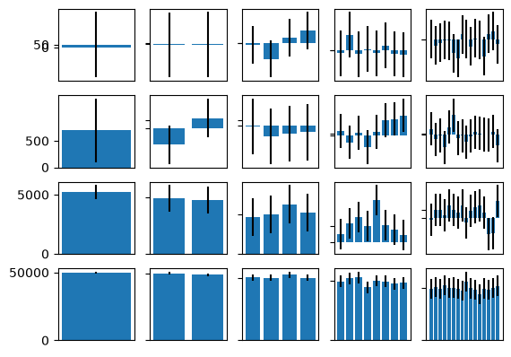
While this wouldn’t be useful for small datasets, with 10,000 rows the results are still good!